In Australia, the relationship between immigration and housing prices has been widely acknowledged across the political spectrum and within our business communities. The common narrative goes something like this: with Australia’s natural population growth in a state of stagnation, immigration has become the primary driver of population growth. When more people settle in Australia, the demand for housing naturally rises. In turn, higher demand for housing pushes up housing prices.
While this narrative has both intuitive appeal and solid academic research to back it up, it is crucial to acknowledge that the housing market is a complex ecosystem influenced by a multitude of factors beyond immigration rates. This includes supply and demand dynamics, interest rates, land availability, construction costs, government policies, and investor activity. While immigration levels may impact housing prices, they are one of many factors that impact the property market.
Nevertheless, analytical investigations by Forecast Global can shed significant light on the temporal dynamics between immigration rates and housing prices. By temporal dynamic, we refer specifically to the time it takes for changes in immigration levels to materialize as changes in housing prices. Understanding this relationship holds relevance from both an investment and a public policy perspective. Investors are eager to know how long it will take for housing prices to increase. While politically, the impact of rising immigration levels on future housing prices can have significant repercussions within various sectors of Australian society.
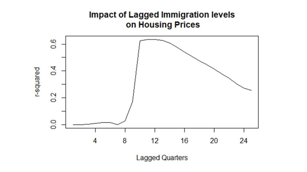
The graph opposite shows “r-squared” values between immigration levels and the national property price index when immigration levels are lagged between 1 and 24 yearly quarters. This graph clearly shows the time delay associated with the impact of immigration levels on housing prices. This impact begins at a lag of around 2.25 to 2.5 years and continues for several years into the future. In other words, it take somewhere between 2.25 and 2.5 years for changes in immigration levels to be felt in the Australian housing market.
Announcements by the Australian Government in September 2022 and May 2023 indicate that Australia’s migrant population is expected to grow by more than 700,000 between the 2022 and 2024 financial years. This number brings Australian immigration growth to an all-time high. By our calculations, this growth will begin to impact the housing market somewhere between late 2024 and early 2025.
This analysis employed a time series approach to data modelling, wherein the two data series used were: 1) Australian Bureau of Statistics National Housing Price Index, and 2) Australian Bureau of Statistics National Immigration Data.
Through meticulous analysis, we have determined that the impact of changes in immigration levels on housing prices takes approximately 2.25 to 2.5 years to materialize. The evidence supporting this conclusion is both compelling and robust. At the heart of this research is the use of a lagged approach to modelling time series data (see figure 1). This involves shifting immigration data backward in time relative to housing prices. By applying this lag, we can explore the relationship between immigration and housing prices in a way that connects past changes in immigration levels to present and future changes in housing prices. For example, if we lag immigration data by 2.5 years against housing prices, we are modelling the impact of immigration levels 2.5 years ago on current housing prices. This time lag allows us to analyse how past changes in immigration levels are associated with current and future changes in housing prices.
To evaluate the strength of our model, we have employed a measure known as an “r-squared” statistic. The r-squared statistic can be used to compare the extent to which changes in one variable are associated with changes in another. Analysts call this “common variance”. If two time series mirror each other (that is, rise and fall in unison), then they are said to have high common variance. On the other hand, if two time series look nothing alike, they are said to have low common variance.