What is uplift modelling?
Targeted marketing is so commonplace, nearly synonymous to online marketing, that consumers have almost come to expect it. Whether those are coupons from your supermarket loyalty scheme, a special one-off discount after deciding to walk away from your full online basket at John Lewis, or a direct mail from your bank telling you about their new credit card offering; you have been targeted.
So how do you identify the individuals who are only likely to click, respond, spend or call after receiving a particular ‘treatment’?
This is called Uplift Modelling.
Propensity or Uplift?
Let’s take the case of a Marketing Director at a retail bank in charge of credit card sales – one of the tools at their disposal to drive sales is a monthly Direct Mail (“DM”) campaign. Even in the unlikely event they would get budget approved to send every customer a communication, it’s obvious that makes no sense. Even if the cost of the treatment is minimal, other costs are likely to play a role, such as taking up valuable communications real estate as contact rules apply or the cost of possibly annoying customers with irrelevant product pushes.
A common flaw in designing such targeted systems is simply using the wrong metric to optimise. This can result in competing incentives, between the marketing team being incentivised by high response rates (propensity), and the product director who cares about total monthly sales (uplift); DM campaign or otherwise. We can see that uplift and propensity are closely related, and uplift is essentially a predictive modelling technique which models the incremental response of a treatment on customer behaviour. However, whereas propensity modelling is concerned with modelling the response to our DM campaign, uplift modelling attempts to quantify the incremental response as a direct result of the email.
Intuitively, sending out a DM campaign is going to increase the overall response rate, positive average uplift. This uplift is unlikely to be uniformly distributed across all customers. In fact, we would expect some customers to be much more likely to respond positively when treated whereas for others the letter makes no difference at all. This is the beauty of uplift modelling; the models are designed to tell us who to target to maximise incremental profits from our DM campaign.
How can you measure uplift?
Uplift modelling is part of a larger subset of statistical modelling techniques attempting to draw causal inferences. This is a difficult question, as traditional statistical models, or in fact, most Machine Learning models in general are concerned with correlation and advanced curve fitting. Stats 101 teaches everyone how ‘correlation does not imply causation’, but observational data does not lend itself to strictly causal inferences. Machine Learning is typically concerned with modelling the observational conditional probability distribution p(y|x) rather than the interventional one p(y|do(x)), as referenced in Judea Pearl’s book, The Book of Why.
As discussed in The Art of Statistics by David Spiegelhalter, Randomised Control Trials give the best framework for drawing causal inferences, and details best statistical practices for trial design. Randomised Trials are commonplace in fields such as medicine, however a large proportion of statistical modelling or datasets might not lend themselves well to that approach. The major exception here is perhaps the online world, where A/B/n type testing is common, and experiments can be run very quickly at huge scale. It’s common knowledge that these techniques are continuously employed by well-known platforms such as Amazon, booking.com and Skyscanner.
If Randomised Trials are not possible for whatever reason, there is an entire field of study concerned with drawing causal conclusions. Examples of such techniques are Structural Equation Models and Bayesian Networks. They usually involve some form of a-priori constraint setting. You can get an introduction to the field here in a great Causal Inference book by Judea Pearl et al.
Fortunately, we have had the luxury of being able to design randomised trials with our clients on several occasions. Each customer is randomly allocated a (particular) treatment, others a control, and we assess the treatment effect across our customers using ‘standard’ uplift models.
Uplift remains a quantity we cannot observe at the individual level. It’s as simple as: you cannot be given both the treatment and the control in the same experiment. This has implications for modelling and evaluation.
How do we model Uplift?
Direct Modelling
There are two main approaches here – direct modelling and indirect modelling. The main difference between the two approaches stems from how we measure and evaluate uplift models.
In direct modelling, we are “directly” modelling the difference in probabilities between two distinct groups. There are many approaches to do so, with almost all of them relying on tree-based algorithms, slightly altered to accommodate uplift modelling.
Tree-based models are ideal as they naturally model at group level by iteratively splitting a group into a further two groups with every splitting decision.
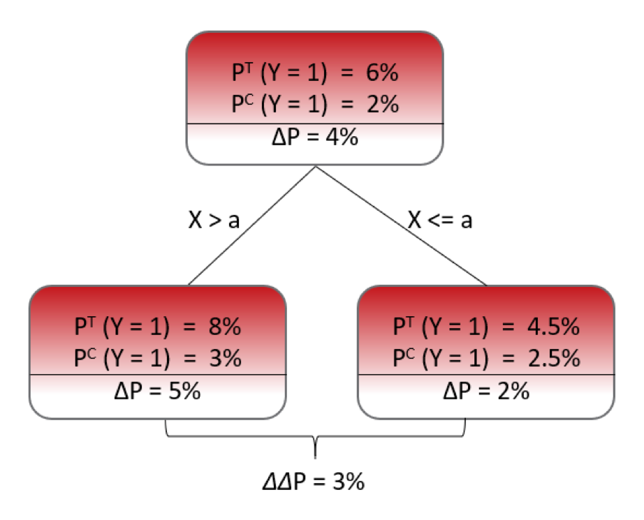
Whereas traditional tree-based models are designed to split the data into smaller and smaller homogeneous groups, uplift models instead are designed to split our customers into heterogeneous groups each time they split (by maximising a measure of uplift). They do so use certain splitting criterions, such as Kullback-Leibler divergence, Euclidean Distance, p-value or Chi-squared Distance. Like traditional tree-based methods, hundreds of trees would be fitted in an ensemble fashion.
The image below shows a simplified Uplift tree grown to depth 1.
Indirect Modelling
Indirect Uplift modelling techniques (meta-learners) are regular response models that are then re-purposed to infer uplift and can be based on any base algorithm. We’re not attempting to optimise some measure of uplift directly and are instead modelling the expected value of the response, for different treatments.
For our DM campaign, we would compute the probability that the customer is going to take the credit card if we send the DM and the probability of taking the product if we do not send the DM. The difference between the two estimated probabilities is the estimated uplift. Practically speaking, this can be a two-model approach (separate model fitted to all control / treatment groups) or a unified model (single model with the allocated treatment part of the feature space). For a more nuanced discussion on different indirect learners (nuanced ways of doing A – B), we refer to the excellent documentation of the fantastic CausalML.
Evaluation of Uplift Models
Remember that we cannot observe uplift directly as it’s impossible to both get the DM campaign and not get it. This not only determines how we go about building models, but also how we can evaluate how well the model performs.
This means that common evaluation metrics for classification problems such as Precision, Recall or Accuracy are not useful to us out-of-the-box and we need to use non-standard metrics to evaluate model performance. Again, these evaluation metrics are focused on using group-level reporting to overcome manyof the issues. We use two intuitive graphs to explain how you could go about evaluating these models.
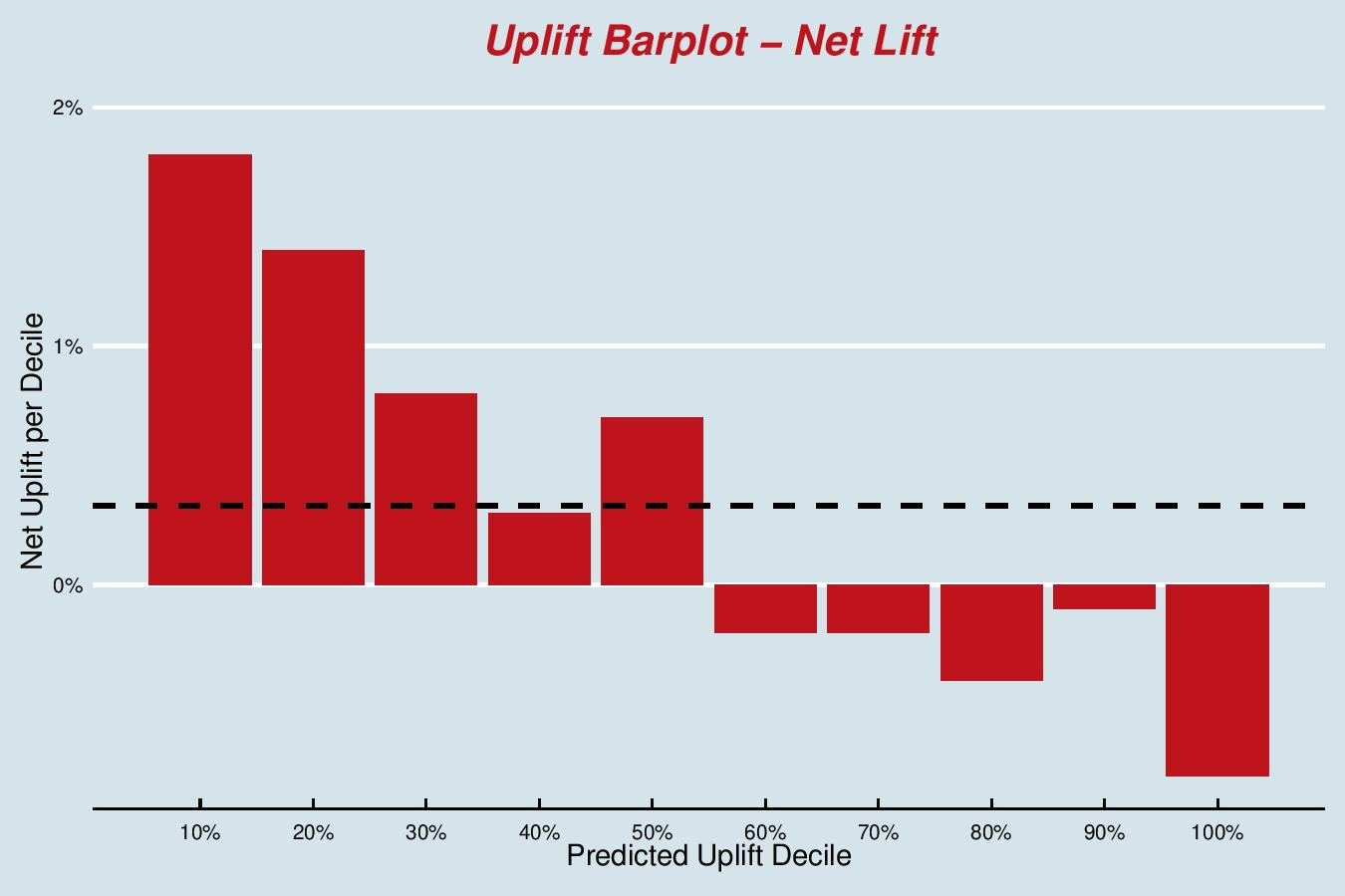
In the Qini barplot, you can see the actuals of net lift for each decile of predicted uplift; the deciles providing the grouping. This model is performing very well – we see a monotonically decreasing lift as we go from the best customers to the worst. Note that the bottom 5 deciles have a negative lift, which means that it would be better to not send these customers the DM; it makes them less likely to take the credit card. The average net lift is plotted horizontally, this shows that deciles 1-5 are above the average (4 borderline).
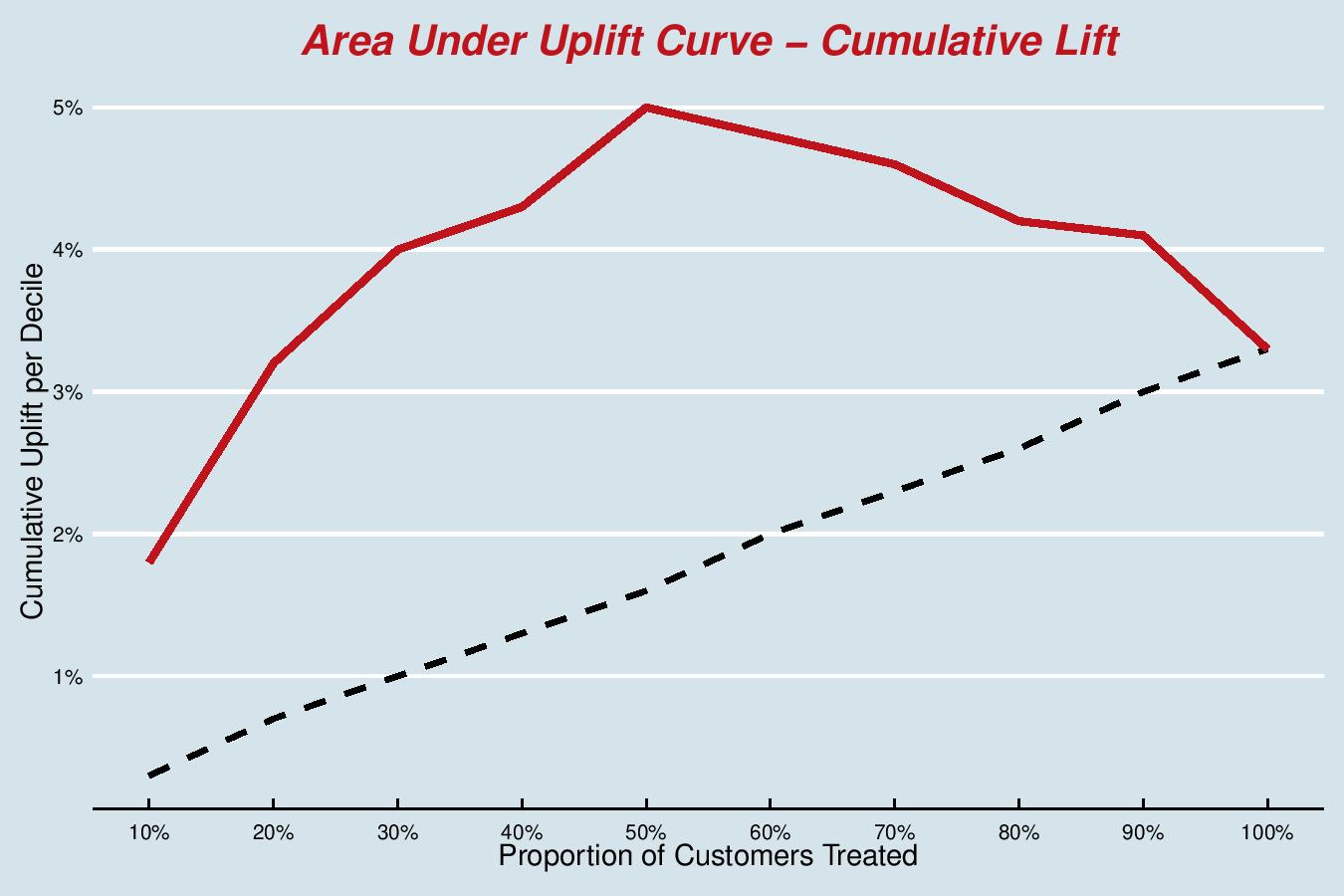
In the Area Under the Uplift Curve, we have the cumulative version of the bar plot. The black line represents the ‘random’ model and the red line is the cumulative lift. Essentially, we’re trying to maximise the area under this curve; if there is one metric to optimise for, then this is most likely the best metric to quote, in the absence of a better understanding of the business application.
We can see that we reach a global maximum at the 5th decile – so in real life, this might be a sensible number to treat, depending on budget and other constraints.
Practical Considerations for Uplift Modelling
Uplift models can be tricky to fit and the evaluation data we used in the section above are certainly fictional. Real-world examples will show a noisier decile profile.
Second Order Effect and Overfitting
We are trying to tease out a second-order effect, the derivative of the target variable with respect to treatment allocation. This second-order effect will most likely be smaller in size than the main effect and, thus, more difficult to pick up. If you consider that the main effect can already suffer from a huge imbalance, the response rate to the DM campaign for our example is likely to be very low single digits. The incrementality due to the treatment is much smaller, which brings noise. When using direct methods, overfitting can be an issue, so watch out for dimensionality, remove noisy (sparse) variables and grow shallower trees.
Variable Selection
Variable selection for uplift modelling can be quite different from standard methods. Here we use metrics like Net Information Value, where we want to maximise the Weights of Evidence between treatment and control. This lets us see the drivers of ‘lift’ before model training.
This can be used for indirect approaches too, giving the best of both worlds, offering the speed of any off-the-shelf algorithm coupled with Direct modelling filtering techniques upfront.
Direct or Indirect
This boils down to several factors. Depending on the technical infrastructure you have available, you might want to stay away from having to rely on packages outside standard distribution of sklearn, in which case indirect is the best choice.
Direct models may take much more time to build and maintain, but have an, at least academic, advantage of modelling the correct quantity. Practically, we often find that the speed of iteration and ease of deployment of indirect models leads to better performance metrics and uptake in the business.
What to optimise
As touched on in the evaluation of uplift models above, for the Marketing Director, deciding to treat all customers would not be a sensible option. First and foremost, there will be budget constraints. There are always options to tune your models to improve performance. For example, if using a direct model, you could tune your Uplift Random Forest based on the out-of-bag Qini co-efficient (Area Under the Uplift Curve) for the top 40% of your population, giving it a custom grid search (for number of trees, number of covariates etc).
Commercial Case Study
At Forecast we worked with a large UK-based telecommunications provider who acquire customers initially at very deep discounts. These initial offers are used by all telecommunications providers, including BT, Virgin and Sky, where you can get up to a 50% reduction on your monthly plan costs for the first year.
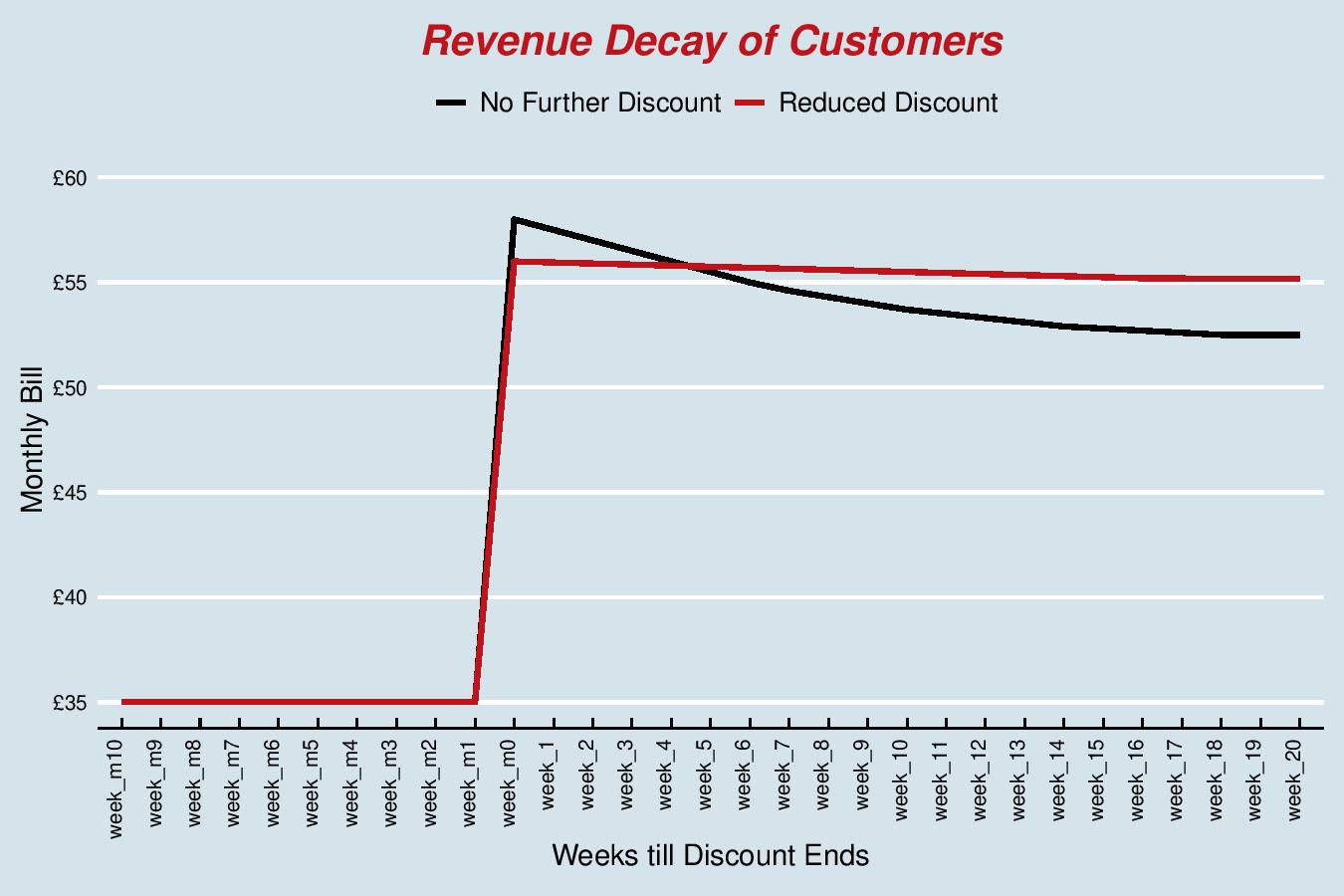
On that one-year anniversary customers would see their bill double, leading to ‘bill shock’ and making them prime candidates for churn. This is reflected by the steep jump in revenue on the chart followed by the revenue decline for the customer base (black line). To mitigate this large churn event, we have been working on pro-active offer extensions. These proactive offers effectively mean the provider will reach out to you with the great news that your offer has been extended for another year. The provider loses out on revenue in the short term where it does not see the hike in price, but the idea is to make up for this loss over time in terms of churn benefits (less churn).
As demonstrated in the chart below, the red line (reduced discount) has a slower rate of decay than the black line (no further discount), meaning they have less customers churning if they offer some form of discount for another year.
Now, the uplift modelling comes in when deciding which customers should be eligible for this proactive treatment. It’s a ‘treatment’ that is not profitable for all, and actually the treatment is not binary either; different levels of offer extensions might be best for different customers.
The telecommunications provider also holds back a pool of customers every month and they’re given random offers (no offer, low offer, medium offer and high offer). Without holding back this pool, they’d never be able to do the following:
- Monitor the performance of our models
- Assess the profitability of the proactive offers
- Update our models to reflect any potential changes in customer behaviour
We hope that through getting to the end of this blog with us, it’s given you some food for thought on implementing uplift modelling in your business. These techniques can be tricky to implement in real life; however, their benefits far outweigh the costs of implementation. We’ve seen huge improvements in targeted outreach for clients, and a better overall understanding of why customers behave how they do.