Numerical Interpretation of Textual Data: Understanding Vector Representations

To model and analyse any unstructured data (like text), we need to transform it into a vector space, so the machine learning algorithm processes it as a feature of vectors. There has been vast research done on the methodologies used in feature representation of text data, each newer method being more computationally complex and better at representing text. From bag of words as sparse vectors to N-gram representations, pre-trained word embeddings and sub-word level representation, there has been a true evolution when it comes to understanding what a word actually means. We will give a general definition of a few of these representations and then compare the model performances using two of the methods.

Bag Of Words

The earliest and most basic representation of features from a block of text is a Bag-Of-Words approach (BOW). This method in its simplest form uses the occurrences of words in the document to create a vocabulary that is encoded into vectors for each sentence. A sentence will have a vector with length the same as the number of words in the vocabulary. Let us assume our dataset has three sentences:

1. The weather is cold
2. Cold season is cold
3. The pizza season is here

The vocabulary for these sentences would have the words [‘The’, ‘weather’, ‘is’, ‘cold’, ‘season’, ’pizza’, ‘here’]. In a one-hot-encoding model, we would create vectors for each sentence of the size of the vocabulary, and for each word present in the sentence, we would have a number. So, for the three sentences, we would get [1,1,1,1,0,0,0], [0,0,2,1,1,0,0], [1,0,1,0,1,1,1] as the encoded vectors. This approach counts the occurrences of each word and encodes the information to words. For a large dataset, the vocabulary size will be massive, and each sentence would have lots of zeroes in them. Such vectors with large sizes and little information are called sparse vectors. This is one of the two major drawbacks of the BOW model, the other being the lack of semantic context encoded in the vectors.

Another approach to represent words in a dataset is using the Term frequency- Inverse Document Frequency (TF-IDF). Instead of the word occurrence counts, it uses the relative frequency of each word in a sentence and in all the sentences in our dataset. The TF calculates local importance of a word and the IDF calculates the dataset importance.

TF = number of occurrence of word in sentence / total words in that sentence
IDF = log (total number of sentences / sentences with the word.)

In our example sentences, the TF of “cold” in the first sentence is 1, while as in second one is 0.5. The IDF value of “cold” in all three sentences is log (3/2) = 0.176. The TF-IDF value for “cold” in 1) is 0.5×0.176. Although this approach models the relative importance of each word better, it still requires large sparse vectors and takes up computational resources while modelling.

When it comes to semantics, the BOW / TF-IDF model does not evaluate the context and meaning of words when encoding them into vectors. The word “bank” will have a specific BOW vector, but it could mean the “river-bank” or the “financial institution”, both of which are used in different contexts and sentiments. To maintain some concept of context we can, in addition to words, use N-grams as separate words in the vector. An N-gram is the combination of any N-words; examples of bi-grams from the above sentences would be “the weather” and “cold season” and “season is”. This only exaggerates the dimensionality problem.

Word Embeddings

A major improvement in modelling context in the word vectors was achieved as a result of using word embeddings as mathematical encodings of words based on their frequency of occurrence with each other. Like the BOW method, word embeddings also generate a fixed length vector for each smallest unit of text, however they model word similarities based on context on the training data. The word “car” and “engine” will have vectors that are close to each other in the vector space because they are used in similar or same contexts. The first option is to train the word embeddings on our dataset prior to using them for language modelling, word prediction or sentiment analysis tasks. This will have a vector space that corresponds to the words we have in our corpus. The second option would be to use pre-trained open-source word embeddings. Both these approaches create N- dimensional vectors for each word, where N is selected based on our computational resources or targets. Words with similar contexts and meanings will be closer to each other in the vector space, and words that are opposite in meaning will have a large Euclidean distance/ low similarity score between them. We will use a basic neural network model that performs sentiment analysis as an example to compare the performance difference in using pre-trained embeddings vs training our own embeddings.

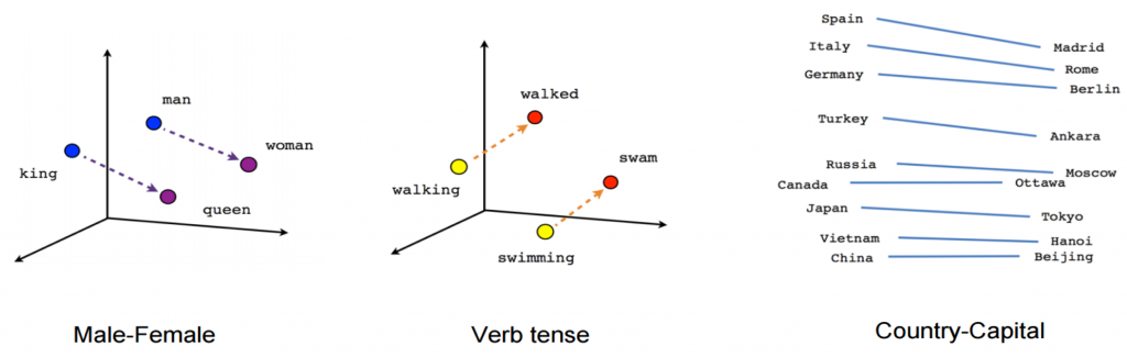
Word embeddings form the first layer of the neural network. Word2Vec was the first embedding that modelled the context of each word and resulted in similar numerical representations for closely-related words. Word2Vec used a neural network to train weights for the input layers to predict a closely related word (“engine”) given a prior word (“car”). The resulting weights are then used as vectors for the word “car”. This ensures the spatial proximity of words used in similar context as shown in the example diagram below. We can see that the verbs in different tenses as well as correlated/similar words occur close to each other in a 3-dimensional vector space representation.

Word2Vec assumes a skip-gram model, where it has a current word as an input and predicts the context, while another pre-trained embedding called GloVe uses the opposite approach called Continuous Bag of Words (CBOW) where it knows the context of a word to predict the word itself.

GloVe constructs a co-occurrence matrix for the context words that count the occurrences of words in contexts rather than in a sentence or document. For the word “north”, the GloVe word embedding calculates the cosine similarities of “west”, “east”, “south” as 0.99, 0.979, 0.986. Similarly, for the word “physics”, it calculates a similarity score of 0.894, 0.889, 0.888 for “biology”, “chemistry”, “quantum” respectively (from a range of 0-1). We will be using GloVe pre-embeddings to compare against having our own embeddings. Let us go through the process we take to do so.

We look at classifying tweets tagged to major US airline companies  into positive, neutral and negative sentiments. We used the embedding layer in Keras to create our own word embeddings from the training data, and alternatively use the GloVe word embeddings with the dimension of 100 vectors. First, we tokenize the tweets into words, and remove the commas, separators, punctuations etc. The next step involves removing stop words from our data. Stop words include most commonly used phrases/words in the corpus that do not have much contextual and meaningful value to the sentence (“and”, ”the”, “or” etc).

stopwords_list = stopwords.words('english') 
whitelist = ["n't", "not", "no"] 
words = input_text.split() 
clean_words = [word for word in words if (word not in stopwords_list or word in 
whitelist) and len(word) > 1] 
return " ".join(clean_words)

We split the dataset into train and test sets, where the test set is going to be used to evaluate the model performance and pad the tweets, so each tweet has the same number of words.

X_train, X_test, y_train, y_test = train_test_split(df.text, df.airline_sentiment, 
test_size=0.1, random_state=37)
X_train_seq_trunc = pad_sequences(X_train_seq, maxlen=MAX_LEN)
X_test_seq_trunc = pad_sequences(X_test_seq, maxlen=MAX_LEN)

We create our embedding model to generate the word embeddings on this tweet dataset and then use these embeddings as the first layer to our neural network to calculate the accuracy of the predicted sentiment on the test dataset.

emb_model = models.Sequential()
emb_model.add(layers.Embedding(NB_WORDS, 8, input_length=MAX_LEN))
emb_model.add(layers.Flatten())
emb_model.add(layers.Dense(3, activation='softmax'))

This model results in an accuracy of 80.53% on the test set, which is quite a good number given the small size of the vocabulary due to less words in the tweets. Twitter data on its own has smaller sentences, lesser context, and far more complex sentiment in the form of non-textual characters. We then look at GloVe pre-embeddings, which are trained on a much larger dataset and then used with custom number of vector dimensions.

glove_model = models.Sequential()
glove_model.add(layers.Embedding(NB_WORDS, GLOVE_DIM, input_length=MAX_LEN))
glove_model.add(layers.Flatten())
glove_model.add(layers.Dense(3, activation='softmax'))

This method results in a 78.21% accuracy over test set classification. There is room for improvement in either methodologies by changing the neural network architecture to recurrent or convolutional to assess the tweet content relationship to a more granular level, but our main takeaway here is that using pre-trained embeddings will not always improve our model performance. We might think that a pre-trained model being built on an extensive dataset of millions or billions of words, but what we don’t realise is the context of our data as compared to the data embedding is trained on. For example, an embedding trained on a corpus of amazon reviews would not map the relationships between words in a legal document. Context in NLP is a very delicate thing. On a website, “opening” or “creating” an account would mean the same, but in general English, “open” and “create” are not semantically related to each other at all. There is a trade-off between having to choose the usefulness of a pre-embedded words and training our own when we have a relatively smaller dataset to work on. The rule of thumb is that for small data to be analysed, a pre-embedding can generalize well to give us valuable vectors but if we are to work on a large text dataset, it’s better to train our own vector embedding in the correct context of our documents.

There is a wealth of information and research done on text representation for machine learning purposes. You can find a similar high level explanation of word embeddings here and here. You can also find an in depth tutorial on how to get started with Google’s BERT embedding in this blog post. A similar explanation and tutorial on using Word2Vec is also available on the Tensorflow website. If you would like to go into the mathematics behind these word embeddings, you can read the original papers published by the creators of word2vec and GloVe. Give it a go, NLP is quite fun topic to learn about!