Survival analysis is the most underrated and underappreciated statistical tool you can have in your toolbox. Survival analysis refers to statistical techniques used to infer “lifetimes” or time-to-event series. Survival analysis does not ignore the complexities of not having observed the event ‘yet’. The event of interest is sometimes called the “death”, as survival analysis these tools were originally used to assess the effectiveness of medical treatments on patient survival rates during clinical trials. Survival analysis can be applied to many business cases including:
- Time until product failure
- Time until a warranty claim
- Time until customer complaint
- Time from initial sales contact to a sale
- Time from employee hire to either termination or quit
- Time from a salesperson hire to their first sale
Customer churn on the other hand is a critical cost (loss of revenue) to any business and significant efforts exist to minimize this cost. No golden standard methodology exists when it comes to predicting which customers will churn and churn may not be so easy to define in a non-contractual business. Survival analysis can be a useful tool when viewing the churn problem set as a time-to-event problem.
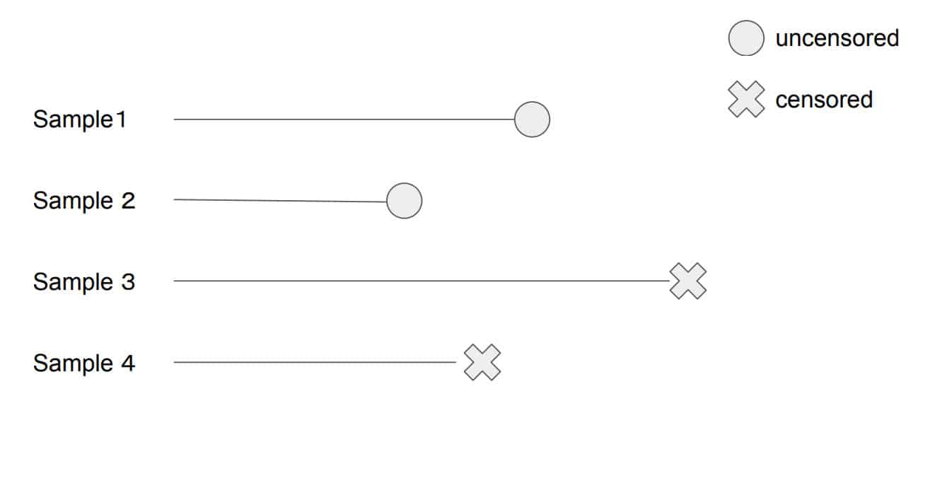
Ordinary regression fails as it fails to account for censored data well. Taking the date of censorship to be the effective last day known for all subjects, or even removing all censored subjects will bias results; dropping unobserved data would under-estimate customer lifetimes.
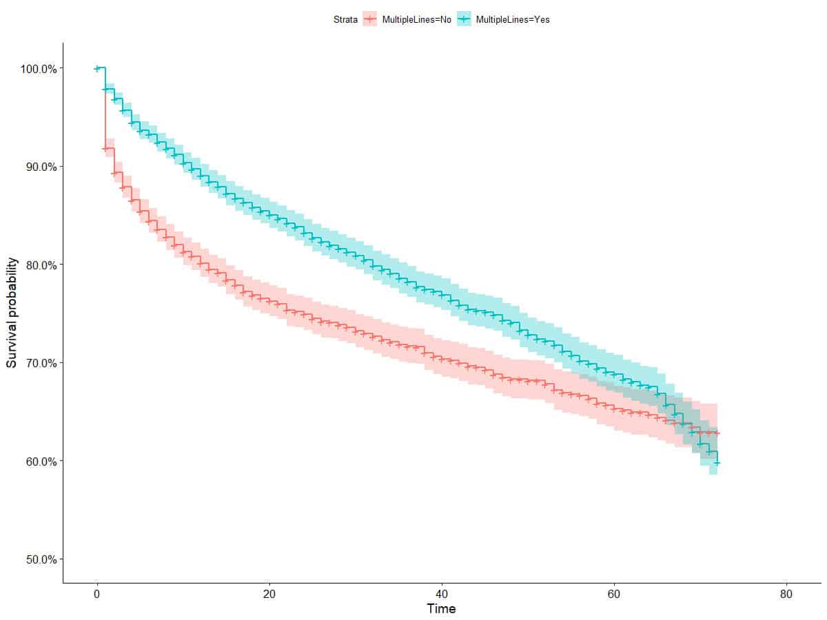
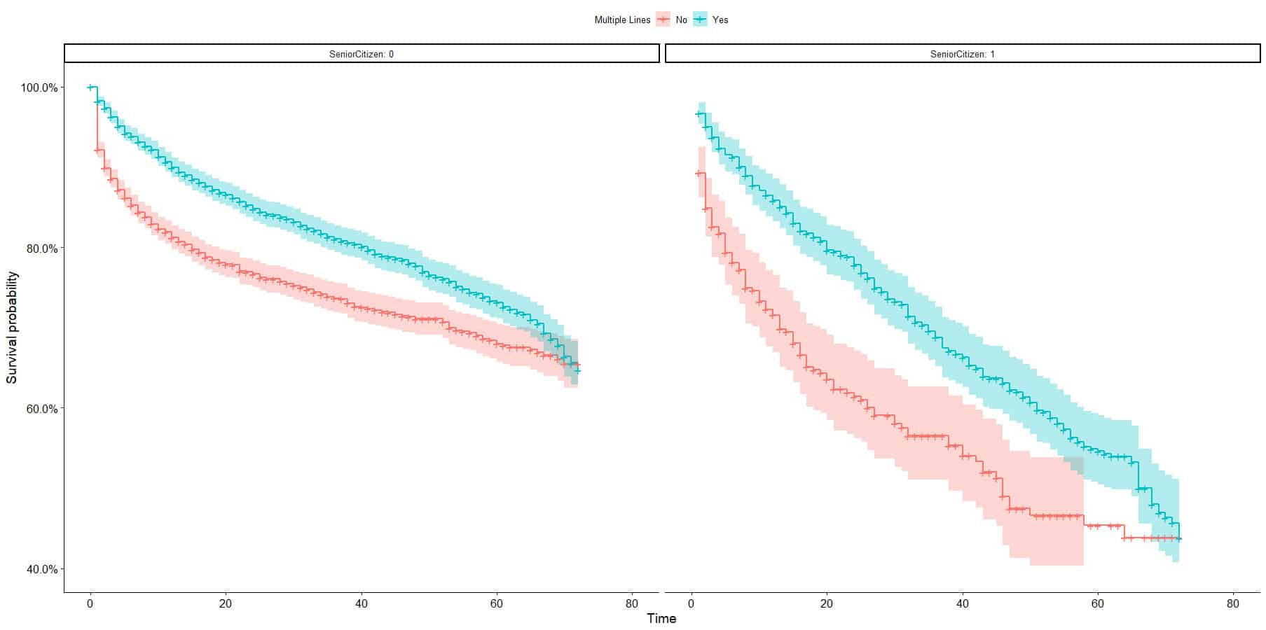
Kaplan-Meier curves are the first tool to exploring survival data and is an easy to use tool to explore how the customer lifetime differs between segments, cohorts or groups. Using the IBM telecommunications dataset we compute the survival curves by segmenting on whether or not the customer has multiple lines (binary variable in the dataset) and we show grouped survival curves that gives us in insight into exploration the lifetime values across two dimensions and their interactions. The first set of curves show that people with Multiple Lines survive at higher rates than those without Multiple Lines. From the confidence intervals on the Kaplan-Meier curves we can see that this difference appears to disappear after about 60 days. The second figure show the same Multiple Lines curves but split by Senior Citizen status. We can see that Senior Citizens appears to survive at much lower rates, but that at least from a visual inspection the effect of Multiple Lines is the same for Senior and non-Senior Citizens; limited interaction effect. Note that the curves have much broader confidence intervals for the Senior Citizens, as this groups is much smaller. The above is simply stating an observation, and this affect may be mitigated by the many other factors that are relevant.
The natural extension of the Kaplan-Meier curves is the Cox regression; the advantage of Cox Regression over Kaplan-Meier is that it can accommodate any number of predictors, rather than group membership only. Visualizing survival curves becomes trickier as more covariates are included, but Cox proportional hazards model can be used for predictions (to generate curves). The former estimates the survival probability, the latter calculates the risk of death and respective hazard ratios.
More recently the Cox proportional hazard model (loss function) has become more widely available after integrating with Machine Learning libraries. Cox hazard modelling has been the domain of regression models for decades, which brings explainability out of the box with readily interpretable coefficients, traditional regression is not as powerful as some machine learning counterparts and cannot account for complex interactions / non-linear patterns / dependencies between ‘covariates’ well, or at all.
To use the powerful XGBoost technique for survival analysis, we will present a very quick demo to showcase how well the two integrate. We will use data from NHANES I with follow-up mortality data from the NHANES I Epidemiologic Follow-up Study. We first import the relevant packages, obtain the data and create the necessary XGB matrix objects.
import shap
import xgboost
from sklearn.model_selection import train_test_splitX,y = shap.datasets.nhanesi()
xgb_full = xgboost.DMatrix(X, label=y)

X_train, X_test, y_train, y_test = train_test_split(X, y, test_size=0.15, random_state=42)
xgb_train = xgboost.DMatrix(X_train, label=y_train)
xgb_test = xgboost.DMatrix(X_test, label=y_test)
We set the training parameters. All that is required is the correct specification of the objective function. And the model can be trained.
watchlist = [(xgb_train, 'train'), (xgb.DMatrix(X_test, label = y_test), 'test')]

params = {
"eta": 0.005,
"max_depth": 2,
"objective": "survival:cox",
"subsample": 0.8
}
model = xgboost.train(params, xgb_train, 10000, watchlist, early_stopping_rounds=25)
If we are interested in comparing performance between models, using statistics that are model agnostic, the default choice in survival models is the concordance index (C-Harrell statistic). We calculate the C-statistic below.
def c_statistic_harrell(pred, labels):
   total = 0
   matches = 0

   for i in range(len(labels)):
      for j in range(len(labels)):
         if labels[j] > 0 and abs(labels[i]) > labels[j]:
            total += 1
         if pred[j] > pred[i]:
            matches += 1

return matches/total

c_statistic_harrell(model.predict(xgb_test), y_test)
Survival analysis is no longer the domain of medicine only, nor is survival analysis restricted to Cox regression. It is an incredibly powerful tool that is heavily underrated, as it is simply forgotten about. Challenges that are classic time-to-event problems are easily misrepresented as regression problems. In particular, Customer Lifetime Value projects might benefit greatly from a survival analysis approach to modelling churn behaviour.