Model interpretation has been and is becoming even more important in the context of human decision making based on model outcomes, artificial intelligence and model scrutiny. We should distinguish between understanding how predictors affect the variable of interest and how these predictors may have complex, non-linear interdependency structures and explaining the contrition of various predictors to individual model outcomes, i.e. individualised outcome attribution. If understanding the model’s decision making is required under a compliance setting, the latter is certainly required, to a high degree of confidence. This article is one of a few in a series about understanding Machine Learning predictions and focuses on the latter problem set, decomposing individual predictions using LIME.
Local surrogate models are interpretable models that are used to explain individual predictions of black box machine learning models. Local interpretable model-agnostic explanations (LIME) (Ribeiro, M.T., Singh, S. and Guestrin, C., 2016) are a particular implementation of local surrogate models. Surrogate models are trained to approximate the predictions of the underlying black box model. Instead of training a global surrogate model, LIME trains local surrogate models to explain individual predictions.
Suppose you have a black box model of any kind that takes input data points and outputs the predictions. You can query the box as often as you please with new input data. Your objective becomes understanding why the machine learning model made a certain prediction. LIME looks at what happens to the predictions of your black box when you feed variations of your data into the machine learning model. LIME generates a new dataset consisting of permuted samples and the corresponding predictions of the black box model. On this new dataset LIME then trains an interpretable model and the interpretable model can be any algorithm that is considered interpretable, such as (lasso) regression or decision trees. The fitted model should be a good approximation to the black box model predictions locally.
When you replace the underlying machine learning model, the same local model can still be used for interpretations. Suppose the people looking at the explanations understand decision trees best. Because you use local surrogate models, you use decision trees as explanations without actually having to use a decision tree to make the predictions. For example you could use a neural network. If it turns out a XGBoost model predicts even better, you can change the black box model and leave the LIME intact.
Using regression of shallow decision trees, the explanations brief making human-friendly explanations. LIME is therefore most useful in applications where the explanation is needed by a lay person, or part of a brief overview. It will not be a complete attribution, but it will go a long way even in scenarios where you might be (legally) required to fully explain individual predictions.
The explanations created with local surrogate models can use other features than the original model. This can be a big advantage over other methods, especially if the original features cannot be interpreted. A regression model can rely on a non-interpretable transformation of some attributes, but the explanations can be created with the original attributes.
Using the iris dataset, we build a simple Random Forest model that achieves an accuracy of 96%. We initiate our LIME (Ridge Regression) to explain the predicted values using all four original variables, for the class with the highest predicted probability.
import lime
import lime.lime_tabular
import pandas as pd
import numpy as np
import sklearn.ensemble
import xgboost as xgb
from sklearn.preprocessing import LabelEncoder
from sklearn.model_selection import train_test_split
from sklearn import datasets


iris = sklearn.datasets.load_iris()
train, test, labels_train, labels_test =
sklearn.model_selection.train_test_split(iris.data, iris.target,
train_size=0.80, random_state=65)
rf = sklearn.ensemble.RandomForestClassifier(n_estimators=500)
rf.fit(train, labels_train)
print(sklearn.metrics.accuracy_score(labels_test, rf.predict(test)))


explainer = lime.lime_tabular.LimeTabularExplainer(train,
feature_names=iris.feature_names, class_names=iris.target_names,
discretize_continuous=True)


rows = [1, 8, 11, 3]
for row in rows:
   exp = explainer.explain_instance(test[row], rf.predict_proba, num_features=4,
   top_labels=1)
   exp.show_in_notebook(show_table=True, show_all=False)
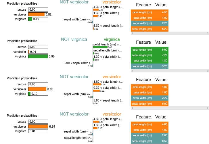
For four rows of data, four instances, we have generated the LIME explainers. On the left we can see how each of the four instances have been classified; the model attached an 81% probability to the first instance being ‘versicolor’ and attached a 96% probability to the second instance being ‘virginica’. The middle column of the explainer demonstrates the core of the LIME explainer and breaks down the predicted probability into contributions for each predictor.
Machine Learning models find their way into all aspects of the work environment and ever more it is important that the model is not only understandable by ML experts, but by human decision makers. LIME is one tool that can be used to simplify the model’s decision for individual predictions. LIME allows the prediction to be decomposed into interpretable components, allowing attribution for lay people or as part of a model review.